Advanced usage

The requirements to follow the tutorial are the same than for the basic example.

To start, let us first import Matplotlib, MDAnalysis and MAICoS, load the trajectory and create our groups.

import logging

import matplotlib.pyplot as plt
import MDAnalysis as mda

import maicos

u = mda.Universe("slit_flow.tpr", "slit_flow.trr")

group_H2O = u.select_atoms("type OW HW")
group_O = u.select_atoms("type OW")
group_H = u.select_atoms("type HW")
group_NaCl = u.select_atoms("type SOD CLA")

Uncertainity estimates

Let us use the maicos.DensityPlanar class to extract the density profile of the group_H2O along the (default) \(z\) axis by running the analysis:

dplan = maicos.DensityPlanar(group_H2O).run()

zcoor = dplan.results.bin_pos
dens = dplan.results.profile

# MAICoS estimates the uncertainity for each profile. This uncertainity is stored inside
# the `dprofile` attribute.

uncertainity = dplan.results.dprofile

# Let us plot the results also showing the uncertainities

fig, ax = plt.subplots()

ax.errorbar(zcoor, dens, 5 * uncertainity)

ax.set_xlabel(r"z coordinate ($\rm Å$)")
ax.set_ylabel(r"density H2O ($\rm u \cdot Å^{-3}$)")


fig.show()

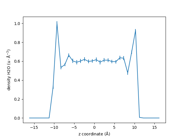
For this example we scale the error by 5 to be visible in the plot.

The uncertainity estimatation assumes that the trajectory data is uncorraleted. If the correlation time is too high or not reasonably computable a warning occurs that the uncertainity estimatation might be unreasonable.

maicos.DensityPlanar(group_H2O).run(start=10, stop=13, step=1)

/home/runner/work/maicos/maicos/src/maicos/core/base.py:566: UserWarning: Your trajectory is too short to estimate a correlation time. Use the calculated error estimates with caution.
  self.corrtime = correlation_analysis(self.timeseries)

<maicos.modules.densityplanar.DensityPlanar object at 0x7f8afbab6210>

Improving the Results

By changing the value of the default parameters, one can improve the results, and perform more advanced operations.

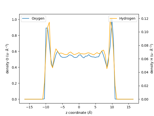
Let us increase the spatial resolution by reducing the bin_width, and extract two profiles instead of one:

• one for the oxygen atoms of the water molecules,

• one from the hydrogen atoms:

dplan_smaller_bin = []
for ag in [group_O, group_H]:
    dplan_smaller_bin.append(
        maicos.DensityPlanar(ag, bin_width=0.5, unwrap=False).run()
    )

zcoor_smaller_bin_O = dplan_smaller_bin[0].results.bin_pos
dens_smaller_bin_O = dplan_smaller_bin[0].results.profile

zcoor_smaller_bin_H = dplan_smaller_bin[1].results.bin_pos
dens_smaller_bin_H = dplan_smaller_bin[1].results.profile

Let us plot the results using two differents \(y\)-axis:

fig, ax1 = plt.subplots()

ax1.plot(zcoor_smaller_bin_O, dens_smaller_bin_O, label=r"Oxygen")
ax2 = ax1.twinx()
ax2.plot(zcoor_smaller_bin_H, dens_smaller_bin_H, label=r"Hydrogen", color="orange")

ax1.set_xlabel(r"z coordinate ($Å$)")
ax1.set_ylabel(r"density O ($\rm u \cdot Å^{-3}$)")

ax2.set_ylabel(r"density H ($\rm u \cdot Å^{-3}$)")
ax1.legend()
ax2.legend(loc=1)

fig.show()

AnalysisCollection example

When multiple analysis are done on the same trajectory, using AnalysisCollection can lead to a speedup compared to running the individual analyses, since the trajectory loop is performed only once. Let us imagine that we want to compute the density of both the oxygen and hydrogen group:

dplan_array = []
for ag in [group_O, group_H]:
    dplan_array.append(maicos.DensityPlanar(ag, unwrap=False))

Now instead of running them in a loop, we will create an AnalysisCollection object:

collection = maicos.core.AnalysisCollection(*dplan_array).run()

/home/runner/work/maicos/maicos/examples/basics/advanced-usage.py:130: UserWarning: `AnalysisCollection` is still experimental. You should not use it for anything important.
  collection = maicos.core.AnalysisCollection(*dplan_array).run()

Now we can now access the result as before:

zcoor_smaller_bin_O = dplan_smaller_bin[0].results.bin_pos
dens_smaller_bin_O = dplan_smaller_bin[0].results.profile

zcoor_smaller_bin_H = dplan_smaller_bin[1].results.bin_pos
dens_smaller_bin_H = dplan_smaller_bin[1].results.profile

Access to all the Module’s Options

For each MAICoS module, they are several parameters similar to bin_width. The parameter list and default options are listed in the module’s documentation, and can be gathered by calling the help function of Python:

help(maicos.DensityPlanar)

Help on class DensityPlanar in module maicos.modules.densityplanar:

class DensityPlanar(maicos.core.planar.ProfilePlanarBase)
 |  DensityPlanar(
 |      atomgroup: mda.AtomGroup,
 |      dens: str = 'mass',
 |      dim: int = 2,
 |      zmin: float | None = None,
 |      zmax: float | None = None,
 |      bin_width: float = 1,
 |      bin_method: str = 'com',
 |      grouping: str = 'atoms',
 |      sym: bool = False,
 |      refgroup: mda.AtomGroup | None = None,
 |      unwrap: bool = True,
 |      pack: bool = True,
 |      jitter: float = 0.0,
 |      concfreq: int = 0,
 |      output: str = 'density.dat'
 |  ) -> None
 |
 |  Cartesian partial density profiles.
 |
 |  Calculations are carried out for ``mass``
 |  :math:`(\rm u \cdot Å^{-3})`, ``number`` :math:`(\rm Å^{-3})`, partial ``charge``
 |  :math:`(\rm e \cdot Å^{-3})` or electron :math:`(\rm e \cdot Å^{-3})` density
 |  profiles
 |  along certain cartesian axes ``[x, y, z]`` of the simulation
 |  cell.
 |  Cell dimensions are allowed to fluctuate in time.
 |
 |  For grouping with respect to ``molecules``, ``residues`` etc., the corresponding
 |  centers (i.e., center of mass), taking into account periodic boundary conditions,
 |  are calculated. For these calculations molecules will be unwrapped/made whole.
 |  Trajectories containing already whole molecules can be run with ``unwrap=False`` to
 |  gain a speedup. For grouping with respect to atoms, the ``unwrap`` option is always
 |  ignored.
 |
 |  For the correlation analysis the central bin
 |  (:math:`N / 2`) of the 0th's group profile is used. For further information on the correlation analysis please
 |  refer to :class:`AnalysisBase <maicos.core.base.AnalysisBase>` or the
 |  :ref:`general-design` section.
 |
 |  Parameters
 |  ----------
 |  atomgroup : MDAnalysis.core.groups.AtomGroup
 |      A :class:`~MDAnalysis.core.groups.AtomGroup` for which the calculations are
 |      performed.
 |  dens : {``"mass"``, ``"number"``, ``"charge"``, ``"electron"``}
 |      density type to be calculated.
 |
 |  dim : {0, 1, 2}
 |      Dimension for binning (``x=0``, ``y=1``, ``z=1``).
 |  zmin : float
 |      Minimal coordinate for evaluation (in Å) with respect to the center of mass of
 |      the refgroup.
 |      If ``zmin=None``, all coordinates down to the lower cell boundary are taken into
 |      account.
 |  zmax : float
 |      Maximal coordinate for evaluation (in Å) with respect to the center of mass of the
 |      refgroup.
 |      If ``zmax = None``, all coordinates up to the upper cell boundary are taken into
 |      account.
 |  bin_width : float
 |      Width of the bins (in Å).
 |  bin_method : {``"com"``, ``"cog"``, ``"coc"``}
 |      Method for the position binning.
 |
 |      The possible options are center of mass (``"com"``), center of geometry (``"cog"``),
 |      and center of charge (``"coc"``).
 |  grouping : {``"atoms"``, ``"residues"``, ``"segments"``, ``"molecules"``, ``"fragments"``}
 |      Atom grouping for the calculations.
 |
 |      The possible grouping options are the atom positions (in the case where
 |      ``grouping="atoms"``) or the center of mass of the specified grouping unit (in the
 |      case where ``grouping="residues"``, ``"segments"``, ``"molecules"`` or
 |      ``"fragments"``).
 |  sym : bool
 |      Symmetrize the profile. Only works in combination with ``refgroup``.
 |  refgroup : MDAnalysis.core.groups.AtomGroup
 |      Reference :class:`~MDAnalysis.core.groups.AtomGroup` used for the calculation. If
 |      ``refgroup`` is provided, the calculation is performed relative to the center of
 |      mass of the AtomGroup. If ``refgroup`` is :obj:`None` the calculations are performed
 |      with respect to the center of the (changing) box.
 |  unwrap : bool
 |      When :obj:`True`, molecules that are broken due to the periodic boundary conditions
 |      are made whole.
 |
 |      If the input contains molecules that are already whole, speed up the calculation by
 |      disabling unwrap. To do so, use the flag ``-no-unwrap`` when using MAICoS from the
 |      command line, or use ``unwrap=False`` when using MAICoS from the Python interpreter.
 |
 |      Note: Molecules containing virtual sites (e.g. TIP4P water models) are not currently
 |      supported in MDAnalysis. In this case, you need to provide unwrapped trajectory
 |      files directly, and disable unwrap. Trajectories can be unwrapped, for example,
 |      using the ``trjconv`` command of GROMACS.
 |  pack : bool
 |      When :obj:`True`, molecules are put back into the unit cell. This is required
 |      because MAICoS only takes into account molecules that are inside the unit cell.
 |
 |      If the input contains molecules that are already packed, speed up the calculation by
 |      disabling packing with ``pack=False``.
 |  jitter : float
 |      Magnitude of the random noise to add to the atomic positions.
 |
 |      A jitter can be used to stabilize the aliasing effects sometimes appearing when
 |      histogramming data. The jitter value should be about the precision of the
 |      trajectory. In that case, using jitter will not alter the results of the histogram.
 |      If ``jitter = 0.0`` (default), the original atomic positions are kept unchanged.
 |
 |      You can estimate the precision of the positions in your trajectory with
 |      :func:`maicos.lib.util.trajectory_precision`. Note that if the precision is not the
 |      same for all frames, the smallest precision should be used.
 |  concfreq : int
 |      When concfreq (for conclude frequency) is larger than ``0``, the conclude function
 |      is called and the output files are written every ``concfreq`` frames.
 |  output : str
 |      Output filename.
 |
 |  Attributes
 |  ----------
 |  results.bin_pos : numpy.ndarray
 |      Bin positions (in Å) ranging from ``zmin`` to ``zmax``.
 |  results.profile : numpy.ndarray
 |      Calculated profile.
 |  results.dprofile : numpy.ndarray
 |      Estimated profile's uncertainity.
 |
 |  Notes
 |  -----
 |  Partial mass density profiles can be used to calculate the ideal component of the
 |  chemical potential. For details, take a look at the corresponding :ref:`How-to
 |  guide<sphx_glr_generated_examples_basics_chemical-potential.py>`.
 |
 |  Method resolution order:
 |      DensityPlanar
 |      maicos.core.planar.ProfilePlanarBase
 |      maicos.core.planar.PlanarBase
 |      maicos.core.base.AnalysisBase
 |      maicos.core.base._Runner
 |      MDAnalysis.analysis.base.AnalysisBase
 |      maicos.core.base.ProfileBase
 |      builtins.object
 |
 |  Methods defined here:
 |
 |  __init__(
 |      self,
 |      atomgroup: mda.AtomGroup,
 |      dens: str = 'mass',
 |      dim: int = 2,
 |      zmin: float | None = None,
 |      zmax: float | None = None,
 |      bin_width: float = 1,
 |      bin_method: str = 'com',
 |      grouping: str = 'atoms',
 |      sym: bool = False,
 |      refgroup: mda.AtomGroup | None = None,
 |      unwrap: bool = True,
 |      pack: bool = True,
 |      jitter: float = 0.0,
 |      concfreq: int = 0,
 |      output: str = 'density.dat'
 |  ) -> None
 |      Initialize self.  See help(type(self)) for accurate signature.
 |
 |  ----------------------------------------------------------------------
 |  Readonly properties inherited from maicos.core.planar.PlanarBase:
 |
 |  odims
 |      Other dimensions perpendicular to dim i.e. (0,2) if dim = 1.
 |
 |  ----------------------------------------------------------------------
 |  Methods inherited from maicos.core.base.AnalysisBase:
 |
 |  run(
 |      self,
 |      start: int | None = None,
 |      stop: int | None = None,
 |      step: int | None = None,
 |      frames: int | None = None,
 |      verbose: bool | None = None,
 |      progressbar_kwargs: dict | None = None
 |  ) -> Self
 |      Iterate over the trajectory.
 |
 |      Parameters
 |      ----------
 |      start : int
 |          start frame of analysis
 |      stop : int
 |          stop frame of analysis
 |      step : int
 |          number of frames to skip between each analysed frame
 |      frames : array_like
 |          array of integers or booleans to slice trajectory; ``frames`` can only be
 |          used *instead* of ``start``, ``stop``, and ``step``. Setting *both*
 |          ``frames`` and at least one of ``start``, ``stop``, ``step`` to a
 |          non-default value will raise a :exc:`ValueError`.
 |      verbose : bool
 |          Turn on verbosity
 |      progressbar_kwargs : dict
 |          ProgressBar keywords with custom parameters regarding progress bar position,
 |          etc; see :class:`MDAnalysis.lib.log.ProgressBar` for full list.
 |
 |      Returns
 |      -------
 |      self : object
 |          analysis object
 |
 |  savetxt(self, fname: str, X: np.ndarray, columns: list[str] | None = None) -> None
 |      Save to text.
 |
 |      An extension of the numpy savetxt function. Adds the command line input to the
 |      header and checks for a doubled defined filesuffix.
 |
 |      Return a header for the text file to save the data to. This method builds a
 |      generic header that can be used by any MAICoS module. It is called by the save
 |      method of each module.
 |
 |      The information it collects is:
 |        - timestamp of the analysis
 |        - name of the module
 |        - version of MAICoS that was used
 |        - command line arguments that were used to run the module
 |        - module call including the default arguments
 |        - number of frames that were analyzed
 |        - atomgroup that was analyzed
 |        - output messages from modules and base classes (if they exist)
 |
 |  ----------------------------------------------------------------------
 |  Readonly properties inherited from maicos.core.base.AnalysisBase:
 |
 |  box_center
 |      Center of the simulation cell.
 |
 |  box_lengths
 |      Lengths of the simulation cell vectors.
 |
 |  ----------------------------------------------------------------------
 |  Data descriptors inherited from maicos.core.base._Runner:
 |
 |  __dict__
 |      dictionary for instance variables
 |
 |  __weakref__
 |      list of weak references to the object
 |
 |  ----------------------------------------------------------------------
 |  Class methods inherited from MDAnalysis.analysis.base.AnalysisBase:
 |
 |  get_supported_backends()
 |      Tuple with backends supported by the core library for a given class.
 |      User can pass either one of these values as ``backend=...`` to
 |      :meth:`run()` method, or a custom object that has ``apply`` method
 |      (see documentation for :meth:`run()`):
 |
 |       - 'serial': no parallelization
 |       - 'multiprocessing': parallelization using `multiprocessing.Pool`
 |       - 'dask': parallelization using `dask.delayed.compute()`. Requires
 |         installation of `mdanalysis[dask]`
 |
 |      If you want to add your own backend to an existing class, pass a
 |      :class:`backends.BackendBase` subclass (see its documentation to learn
 |      how to implement it properly), and specify ``unsupported_backend=True``.
 |
 |      Returns
 |      -------
 |      tuple
 |          names of built-in backends that can be used in :meth:`run(backend=...)`
 |
 |
 |      .. versionadded:: 2.8.0
 |
 |  ----------------------------------------------------------------------
 |  Readonly properties inherited from MDAnalysis.analysis.base.AnalysisBase:
 |
 |  parallelizable
 |      Boolean mark showing that a given class can be parallelizable with
 |      split-apply-combine procedure. Namely, if we can safely distribute
 |      :meth:`_single_frame` to multiple workers and then combine them with a
 |      proper :meth:`_conclude` call. If set to ``False``, no backends except
 |      for ``serial`` are supported.
 |
 |      .. note::   If you want to check parallelizability of the whole class, without
 |                  explicitly creating an instance of the class, see
 |                  :attr:`_analysis_algorithm_is_parallelizable`. Note that you
 |                  setting it to other value will break things if the algorithm
 |                  behind the analysis is not trivially parallelizable.
 |
 |
 |      Returns
 |      -------
 |      bool
 |          if a given ``AnalysisBase`` subclass instance
 |          is parallelizable with split-apply-combine, or not
 |
 |
 |      .. versionadded:: 2.8.0
 |
 |  ----------------------------------------------------------------------
 |  Methods inherited from maicos.core.base.ProfileBase:
 |
 |  save(self) -> None
 |      Save results of analysis to file specified by ``output``.

Here we can see that for maicos.DensityPlanar, there are several possible options such as zmin, zmax (the minimal and maximal coordinates to consider), or refgroup (to perform the binning with respect to the center of mass of a certain group of atoms).

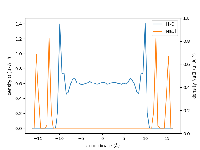
Knowing this, let us re-calculate the density profile of \(\mathrm{H_2O}\), but this time using the group group_H2O as a reference for the center of mass:

dplan_centered_H2O = maicos.DensityPlanar(
    group_H2O, bin_width=0.5, refgroup=group_H2O, unwrap=False
)
dplan_centered_H2O.run()
zcoor_centered_H2O = dplan_centered_H2O.results.bin_pos
dens_centered_H2O = dplan_centered_H2O.results.profile

Let us also extract the density profile for the NaCl walls, but centered with respect to the center of mass of the \(\mathrm{H_2O}\) group:

dplan_centered_NaCl = maicos.DensityPlanar(
    group_NaCl, bin_width=0.5, refgroup=group_H2O, unwrap=False
)
dplan_centered_NaCl.run()
zcoor_centered_NaCl = dplan_centered_NaCl.results.bin_pos
dens_centered_NaCl = dplan_centered_NaCl.results.profile

/home/runner/work/maicos/maicos/src/maicos/lib/math.py:183: RuntimeWarning: invalid value encountered in divide
  (1 - np.arange(1, cutoff) / len(timeseries)) * corr[1:cutoff] / corr[0]
/home/runner/work/maicos/maicos/src/maicos/core/base.py:566: UserWarning: Your trajectory does not provide sufficient statistics to estimate a correlation time. Use the calculated error estimates with caution.
  self.corrtime = correlation_analysis(self.timeseries)

An plot the two profiles with different \(y\)-axis:

fig, ax1 = plt.subplots()

ax1.plot(zcoor_centered_H2O, dens_centered_H2O, label=r"$\rm H_2O$")
ax1.plot(zcoor_centered_NaCl, dens_centered_NaCl / 5, label=r"$\rm NaCl$")

ax1.set_xlabel(r"z coordinate ($Å$)")
ax1.set_ylabel(r"density O ($\rm u \cdot Å^{-3}$)")
ax1.legend()

ax2 = ax1.twinx()
ax2.set_ylabel(r"density NaCl ($\rm u \cdot Å^{-3}$)")

fig.show()

Additional Options

Use verbose=True to display extra informations and a progress bar:

dplan_verbose = maicos.DensityPlanar(group_H2O)
dplan_verbose.run(verbose=True)

  0%|          | 0/201 [00:00<?, ?it/s]
 16%|█▋        | 33/201 [00:00<00:00, 328.63it/s]
 33%|███▎      | 66/201 [00:00<00:00, 327.62it/s]
 49%|████▉     | 99/201 [00:00<00:00, 327.89it/s]
 66%|██████▌   | 132/201 [00:00<00:00, 328.50it/s]
 82%|████████▏ | 165/201 [00:00<00:00, 328.14it/s]
 99%|█████████▊| 198/201 [00:00<00:00, 328.13it/s]
100%|██████████| 201/201 [00:00<00:00, 327.74it/s]

<maicos.modules.densityplanar.DensityPlanar object at 0x7f8afb461450>

MAICoS uses Python’s standard logging library to display additional informations during the analysis of your trajectory. If you also want to show the DEBUG messages you can configure the logger accordingly.

logger = logging.getLogger("maicos")
logger.setLevel(logging.DEBUG)
dplan_verbose.run()
logger.setLevel(logging.NOTSET)

For additional options take a look at the HOWTO for the logging library.

To analyse only a subpart of a trajectory file, for instance to analyse only frames 2, 4, 6, 8, and 10, use the start, stop, and step keywords as follow:

dplan = maicos.DensityPlanar(group_H2O).run(start=10, stop=20, step=2)